R - catch and analyze info on Website

R Programming for beginners

File - new R Script
comments: #

Create a value/vector

1
2
3
4
5
6
7
8
9
10
11
12
13
14
15
16
17
18
19
1+1 => [1] 2
x = 1 + 1 ;
=> [1] 2
x = 1 + 1 => nothing
grades = c(100,90,85,95); grades => [1] (100,90,85,95)
grades + 5=>
- function: class(X) => data types ofunction X(Numeric/Character)
- y = c(5,10,"15",20) ; y is not numerial anymore though only one element is char, now y is chr and change into [1]"5","10","15","20"
- function: char to numeric: y = as.numeric(y) => [1] 5 10 15 20
- function: numeric to char as.character
- Trouble 1: run previous results neccessary; solution: #comments the variable
- Trouble 2: select rows in code=> run only what you want
1
2
3
4
5
6
7
8
9
10
11
12
13
14
15
16
17
18
19
20
21
22
23
24
function table()& summarize() to calculate the frequency of Vector/Matrix
Print some positions of V:
V[1,2] correct into V[c(1,2)]
V[-2] is OK,but not V[-1,-2], it prints positions except positon 2
function sequence: 1:10; seq(1,10);seq(to = 10, from = 1);seq(10,1);seq(from = 1, to = 10, by = +-2)
function repeat: rep("HI",10)
// will not interfere with embedded <a href="#voila2">tags</a>.
NA means sth does not exist
function 把一大组数归纳总结频率table(),转成表as.data.frame(table()),在表里加一些colomn比如Order:cbind.data.frame
function 排序 order()升序,order(-)降序
- Remember 4: Vector[c(1,2,3...)]获取数值,而matrix$..来获取! 注意!
- Remember 5: Vector直接 mean(Vector)就好!
- Remember 1: Variable[1] not V[0] prints the first one
- Remember 2: Variable's name should be combined without space between
- Remember 3: Factors can not be allowed to compare value (=<>)

Metrix:

1
2
3
4
5
6
7
8
9
10
11
12
13
14
15
16
17
18
19
20
21
22
23
24
25
26
function data.frame(v1,v2) , if length ofunction v1 is larger than v2 then v2's vector in metrix will be repeated to fill the space.
add another colomn to metrix: function cbind(data.frame(v1,v2), v3)
1. 先按照要求造个vector,再作为一个colomn加上去!!!!
function colnames/rownames(M) = c("","") to change the names
function M[A,B] Row 1st, colomn 2nd show numbr on that position, A or B can be left empty to show the full colomn/row, B can be 1:2 or c(1,2) both OK!
function: View(metrix) -> show the table
function length, nrow, ncol, head() tail() names() #head rows,
Sum Fuction: sum(data[,5]); sum(data$population)
- function 不是countif和count,是nrow()! : X[X$region==1,] Return all information on states located in only 1(region ==1). nrow()to count .
Add conditions on colomn show only colomn: X[X$region==1,".."or 1 ]
- function data[data$murder==max(data$murder), "state"] return the state ofunction largest murder
function: T/function matrix: data[data$murder, 1]==max(data$murder) not data[data$murder==max(data$murder), ]
function:ifelse()ifelse(data$illiteracy<1, "low","high")
function 提取table的字/标题 names(table), 提取table的数字 numeric(table)

FOR LOOP + 提取colomn + 创建结果为colomn(各个添加)

1
2
3
4
5
6
7
Create a new column “Age.Range”
age = hw1$Age
Age.Range = ""
for( i in 1:length(age)){if (age[i] < 20){Age.Range[i]="Below 20 years"} else if(25> age[i]){Age.Range[i] = "[20-25) years"}else if(30 > age[i]){Age.Range[i] = "[25-30) years"}
else if(30< age[i]){Age.Range[i] = "Above 30 years"}}
Age.Range

import outside data source

1
2
3
4
5
change/get working directory
function getwd(); setwd("D:/AW/MSBA&Programming合集/R");
open and save file: function data= read.csv("statedata.csv")];
{% endcodeblock %}

CODES

1
2
3
4
5
6
7
8
9
10
11
12
13
14
15
16
17
18
19
20
21
22
23
24
25
26
27
28
29
30
31
32
33
34
35
36
37
38
39
40
41
42
43
44
45
46
47
48
49
50
51
52
53
54
55
56
57
58
59
60
61
62
63
64
65
66
67
68
69
{% codeblock lang:R %}
[
x = 1+1
#x
grades = c(100,90, 85, 95)
# grades
classes = c("DS", "ss")
# classes
class(classes)
grades + 5
y = c(5,10,"15",20)
y = as.numeric(y)
#y
#y[1]
#grades[c(1,2,4)]
#grades[-3,-4]
Metrix1 = cbind(data.frame(y,classes),grades)
#View(Metrix1)
rownames(Metrix1) = c("stu1","stu2","stu3","stu4")
View(Metrix1)
nrow(Metrix1)
2:10
seq(1,10)
seq(to = 10, from = 1)
seq(10,1)
seq(from = 1, to = 10, by = 2)
rep("HI",10)
data= read.csv("statedata.csv")
View(data)
tail(data)
sum(data[,5])
sum(data$population)
nrow(data[data$region== 1 ,])
data[data$illiteracy<0.7, "state"]
#data[data$murder==max(data$murder) or data$murder==min(data$murder), "state" ]
data[data$murder==max(data$murder) and data$murder==min(data$murder) ,1]
data[data$murder, 1]==max(data$murder)
data$illiteracyCategory = ifelse(data$illiteracy<1, "low","high")
data[data$illiteracyCategory=="low",] ];
{% endcodeblock %}

conditional Loops in R — Stupid guy

Age.Range = if(hw1$Age < 20){“Below 20 years”} else{
if(25> hw1$Age >= 20){“[20-25) years”}
else{
if(30 > hw1$Age >= 25){“[25-30) years”}
else{“Above 30 years”}}}
错了!为啥???

  1. 因为elseif 应该是 else if
  2. else if 最后一项也是,不能是else 要写清条件

Beginning

So today we gonna come through some simple data analysis to find the most popular clothes ofunction famous brand “Stylenanda”. (Data from http://en.stylenanda.com/)

Step 1: catch info

All the informations we need are the name price, sales and comments ofunction all the clothes.

1
2
3
4
5
6
7
8
9
10
11
Library(rvest)
Library(xml2)
> as<-seq(60,420,60)
> for(s in as){
moda<-read_html("Stylenandas=60&q=%C1%AC%D2%C2%C8%B9&sort=s&style=g&from=sn_1_brand-qp&active=2&industryCatId=50025135&type=pc#J_Filter",encoding="GBK") +dress_name<-html_nodes(moda,'.productTitle a')%>%html_text
dress_name<-html_nodes(stylenanda,'.productTitle a')%>%html_text
dress_price<-html_nodes(stylenanda,'.productPrice em')%>%html_text sale_number<-html_nodes(stylenanda,'.productStatus em')%>%html_text
> the_comment<-html_nodes(stylenanda,'.productStatus a')%>%html_text
+ }
> dress<-data.frame(dressname,dressprice,salenumber,thecomment)

Step 2: Integrate and Standardize our data

1
2
3
4
> library(plyr)
> Unify variable name
dress1<rename(dress1,c(dress_name="dressname",dress_price="dressprice",sale_number="salenumber",the_comment="thecomment")
> Modadress <-rbind(dress,dress1)

We got the output for “Modadress$dressprice” , new column for the dress price

1
2
3
4
[1] ¥399.00299.50749.00699.00112.00306.00298.00649.00
[9] ¥299.00279.00249.00299.50374.50324.50274.50324.50
[17] ¥349.50199.00349.50699.00279.00349.00749.00199.00
[25] ¥299.50324.50349.50349.50349.50324.50324.50299.0

The number ofunction dress sales :

1
2
3
4
5
6
[1] 11981394001019346483618481203
[12] 56657313801808609177616211162348470397
[23] 446364468579666362776770617611791
[34] 154781275111868891677256955114927
[45] 4717501117734798208620492298160846
[56] 90210934580210168891277456955115

Then we need to filter and delete the unnecessary info

1
2
Modadress$dressprice<-gsub("¥","",Modadress$dressprice)
Modadress$salenumber<-gsub("笔","",Modadress$salenumber)

Find their properties

1
2
3
4
5
6
> class(modadress$salenumber)
[1] "factor"
>class(modadress$thecomment)
[1] "factor"
> class(dressprice)
[1] "character"

Change strings into number format:

1
2
3
> Modadress$dressprice<-as.numeric(modadress$dressprice)
> Modadress$salenumber<-as.numeric(modadress$salenumber)
> Modadress$thecomment<-as.numeric(modadress$thecomment)

Step3: Summarize and Visualize data

Summarize data:

1
2
3
4
5
6
group_by(Modadress,priceleve)%>%summarise(price=mean(dressprice,na.rm=T),number=mean(salenumber,na.rm=T),comment=mean(thecomment,na.rm=T))
# A tibble: 2 x 4
priceleve price number comment
<fctr> <dbl> <dbl> <dbl>
1 high 722.5484 117.6774 39.90323
2 normal 316.2674 703.0562 422.12360

Visualize data in chart

1
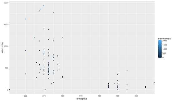
ggplot(Modadress,aes(x=dressprice,y=salenumber,color=thecomment))+geom_point()+scale_x_continuous(expand=c(0,0),breaks=c(100,200,300,400,500,600,700,800,900,1000,1100),labels=c(100,200,300,400,500,600,700,800,900,1000,1100))

From the picture, a lot ofunction clothes fall into the range ofunction 200RMB-400RMB, fewer cost more than 650RMB and none cost 400RMB-650RMB.

Then in order to figure out the sales ofunction clothes falling into each range, we need to recode the price at first and add “pricelevel” variable after that.

1
2
3
4
5
Modadress<-within(Modadres,{
pricelevel<-"NA"
pricelevel[dressprice<450]<-"normal"
pricelevel[dressprice>500]<-"high"
})

Calculate the sales ofunction clothes falling into each range.

1
2
3
4
total<-tapply(Modadress$salenumber,Modadress$pricelevel,sum)
> total
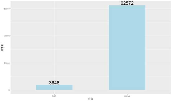
high normal
3648 62572

Differences between two levels ofunction sales are obvious. Now we shall draw into picture to show clearly.

1
2
3
4
z<-c("high","normal")
chart<-data.frame(z,total)
> wtp<-ggplot(chart,aes(x=z,y=total))+geom_bar(stat="identity",fill="lightblue",width=0.5)+geom_text(aes(label=total),vjust=-0.2,colour="black",size=8)
> wtp+xlab("price")+ylab("sales")

Step 4: Get the data we what and rule out others

At first we need to specify the meaning ofunction “Popolar clothers”. The standard I refer to is comment volume and sales volume.

According to the figure above, the lighter the color ofunction the blue dot, the larger the comment volume.

Set 1500 as dividing line and choose the best-selling products.

1
2
filter(Modadress,thecomment>1500)%>%arrange(desc(salenumber))
dressname dressprice salenumber thecomment priceleve

Output:

1 Self-Tie Collar Button-Down Shirt 279 1848 1557 normal
2 Check Pattern Buttoned Back Shirt 199 1621 1822 normal
3 Pre-Damaged Knit Cardigan 249 1203 1647 normal
4 Extended Sleeve Lettering Print Hoodie 399 1198 2059 normal
Thus we got Top4 for most popular clothes:

  1. Self-Tie Collar Button-Down Shirt

  2. Check Pattern Buttoned Back Shirt

  3. Pre-Damaged Knit Cardigan

  4. Extended Sleeve Lettering Print Hoodie

Come on! Just follow this instruction and have a try. Use R to find any info about items ofunction your favorite brand.